Following up on Martin's introduction, this is the second part of our three-part series on process risk simulation. In this article I will show you how the effects of risk occurrence in a business process can be analyzed with simulation.
A significant part of business process management is the analysis and improvement of processes. The analysis may involve many aspects, such as media breaks, added value, throughput times, bottlenecks, resource utilization or cost. An often neglected aspect is risk, in particular operational risk.
Depending on the process, the effects of operational risk can be quite significant and should consequently be taken into consideration during the process analysis. This may help an organization to decide which risks can be accepted and which risks have to be avoided or reduced by means of countermeasures such as process changes or controls. The necessary data can be obtained by means of calculation or simulation methods.
In the context of a business process a risk event can occur during the execution of an activity, regardless of it being caused by the activity or triggered externally. The occurrence of a risk event is not certain but always associated with a probability. And when a risk event occurs, it has undesired consequences, e.g. the loss of money, materials or resources.
The following figure shows how risks appear in an event-driven process chain (EPC). The model, which serves as an example for this article, describes (in an over-simplified way) the process of a credit transfer. Both functions in the sample process have an associated risk which is depicted as a red rectangle. The traits of risks mentioned above are specified in attributes of the risk objects which are not displayed in the figure. In the example the risks only have monetary consequences. Besides the characteristics of risks, several other properties of the process are specified in the model in order to make it more realistic, e.g. processing times or instantiation patterns.
 Figure: Credit transfer process with risk objects
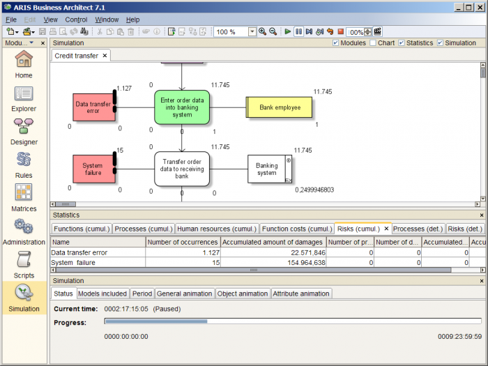
The configured model is simulated with ARIS Business Simulator over a simulation period of ten days in order to get the data for the following analysis. A screenshot of the simulation in action can be found in the following figure.
 Figure: Simulation with ARIS Business Simulator
In the example the main goal of the analysis is to find out how often risk events occurred and how large the losses are due to these occurrences. This information can be found in simulation results as part of the so-called cumulative risk statistics part of which are shown in the following table.
| Risk | Data transfer error | System failure |
|---|---|---|
| Number of occurrences | 4,227 | 45 |
| Accumulated amount of damages | 84,457.51 | 458,378.98 |
The data in the table shows that even though system failures occur much more seldom than data transfer errors, the overall damages are much higher due to the high amount of damages per occurrence. Based on these results alone one would probably try to improve the system reliability in order to reduce the larger share of damages, but if this is the right strategy obviously also depends upon the cost for a reduction of these damages. But since the example does not include controls, there is no information about cost available yet.
In the simple example shown in this article, the use of simulation was not strictly necessary because the information regarding financial losses could also have been obtained through calculation. However, the more complex business processes are, the more difficult their analysis is and the more simulation becomes preferable as a means to support the analysis. It becomes even more useful in case not only financial consequences of risk occurrence are evaluated but also the (temporary) loss of resources which will impact the dynamic behavior of the process. For example, with simulation it would be possible to see if such a resource loss introduces a bottleneck and if the system is able to recover from it once the resource becomes available again.
This concludes the second part of our series about process risk simulation. The next article will demonstrate how controls can be used to reduce the effects of risks.

